General Sigma-Models

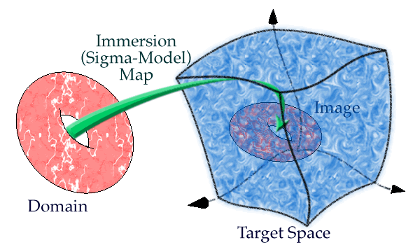
Most succinctly, sigma-models are studies of (constrained) immersion maps. They involve (see also the examples below):

1. a domain (base space), over which the 'independent' variables vary,
2. a target space, over which the dependent variables vary,
3. an immersion map, which specifies where in the target space the image of the domain is,
4. a functional that depends on the immersion map and which governs the constraining of the immersion.

Viewed this way, it is clear that all (theoretical) physics models may be regarded as a sigma-models. Below are a two familiar examples:

The classical mechanics of a single particle:

1. the domain is R¹ (the real axis), over which the (independent) time, t, variable varies;
2. the target space is the actual space, X - usually R³ (the real 3-dimensional space), in which the particle moves;
3. the immersion map is the coordinate function, x(t), which specifies where the particle is at any point in time;
4. the constraining functional is the Hamiltonian action, the minimization of which constrains x(t) to the classical trajectory.

The classical electrodynamics:

1. the domain is R^3,1 (the real spacetime), over which the (say) Cartesian coordinates, x=(x,y,z,t), vary;
2. the target space is the ‘field space’, i.e., the space of gauge potentials modulo gauge transformations;
3. the immersion map is the 4-vector of gauge potentials, A_µ(x), only two (polarizations) of which are physical, and which specify the electromagnetic (vector) field at every point in the 3+1-dimensional spacetime;
4. the constraining functional is the Hamiltonian action, the minimization of which constrains A_µ(x) to the classical trajectory.

The (super)string theory (1st, ‘underlying’ level):

1. the domain is the “world-sheet”, the (punctured Riemann) surface, swept out by the string as it moves in time, and over which the (super)string's spatial and temporal coordinates, (s,t), vary;
2. the target space is the actual spacetime, X (=R^9,1 for simplest superstrings), in which the (super)string moves;
3. the immersion map is the 10-vector, X^µ(s,t), which specifies where each point of the string is at any point in time, and its superpartner, which is a spinor on the Riemann surface (in the 1+1-dimensional sense) and a tangent vector to the actual spacetime, at the point in spacetime to which X^µ(s,t) maps the (s,t) point of the world-sheet.
4. the constraining functional is the Hamiltonian action, essentially the area of the world-sheet; this may contain (arrays of) coupling parameters, the variation of which is governed quantum fluctuations.

The (super)string theory (2nd, ‘effective’ level):

1. the domain is the actual spacetime, X (=R^9,1 for simplest superstrings), in which the (super)string moves;
2. the target space, Y, is the ‘field space’ over which the ‘fields’ (arrays of coupling parameters, at 1st level) vary;
3. the immersion map consists of the various ‘fields’, viewed as functions over X.
4. the constraining functional is the effective Hamiltonian action, for which the terms are obtained as correlation functions at the 1st level.

The (super)string theory (3rd, 'modular' level):

1. the domain is the 'field space', Y, over which the 'fields' (dependent variables at 2nd level) vary;
2. the moduli space, M, over which the parameters (specifying the target space from level 2) vary;
3. the immersion map consists of the various moduli, viewed as functions over Y.
4. the constraining functional is an effective Hamiltonian action, for which the terms are obtained as correlation functions at the 2nd level.

Of special interest to me are supersymmetric sigma-models, where the general framework sigma-models is very importantly aided (in both technical and conceptual sense) by supersymmetry.

© Tristan Hübsch, 2008